EXECUTIVE SUMMARY
We report a simple yet powerful statistical model of county-level voter behavior in the November 2020 presidential election using two main types of data:
(Article republished from Revolver.news)
- County-specific voting data from the five previous presidential elections.
- Selected demographic variables (race and education) plotting how different national voter groups voted differently in 2020 overall.
These two types of predictors allow us to explain over 95% of the variation in county-level votes, and therefore allow us identify which counties (and consequently, states) look substantially anomalous in the 2020 election.
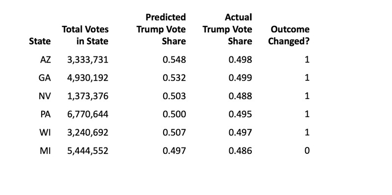
The model provides substantial support for the allegation that the outcome of the election was affected by fraud in multiple states. Specifically, the model’s predictions match the reported results in all other states, i.e. states where no fraud has been alleged, but predicts Trump won majorities in five disputed states (AZ, GA, NV, PA and WI) and 49.68% of the vote in the sixth (MI).
In other words, the reported Biden margin of victory in at least five of the six contested states cannot be explained by any patterns in voter preference consistent with national demographic trends.
SUMMARY OF MAIN ARGUMENTS
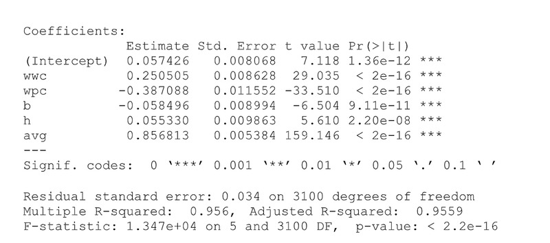
1. Our model explains 96% of county-level variance in Trump’s two-party vote share with four demographic variables (non-college white, college-educated white, black and hispanic) and one historical variable (the average of county-level GOP two-party presidential vote share, 2004-2016). All five variables are highly significant. This reinforces the conclusion that the model is generally a very strong predictor of vote shares, and so deviations from it should be considered surprising.
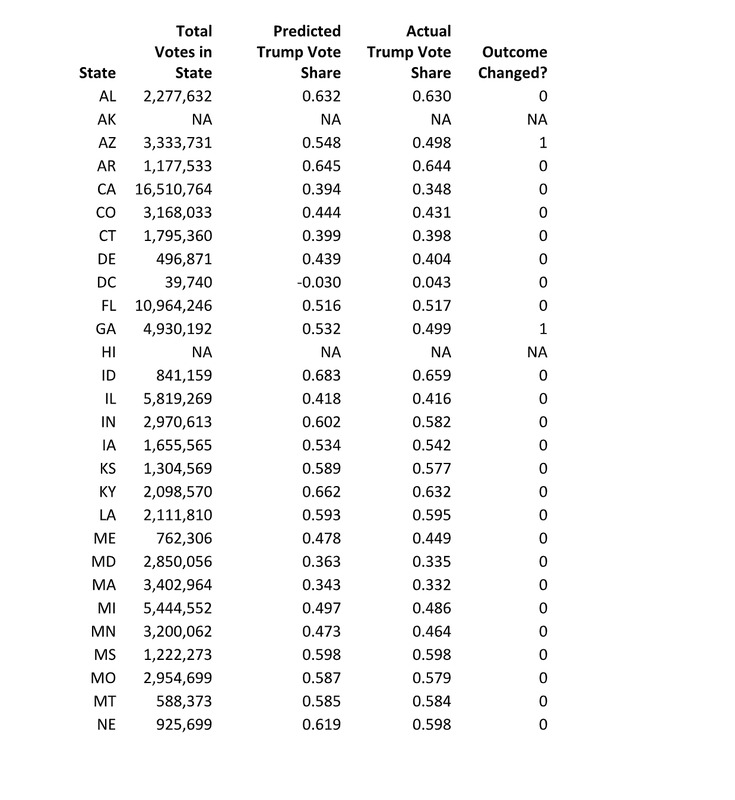
2. Under conservative assumptions, regression analysis shows Trump ought to have won AZ, GA, NV, PA, WI.
[See the end of the article for the full table.]
3. Every one of the contested states shows a larger predicted vote share for Trump than what he actually received. This is surprising, because in any set of observations, random chance might expect some predictions to favor Biden, but none do. In Georgia and Arizona, the model does not predict a narrow race, but a decisive Trump victory; the size of the anomaly is (much) larger than the reported margin of victory.
4. The model also performs well in battleground states that have not been contested, and thus where the election was presumably clean. Every one of these is correctly predicted, including both battleground states that voted for Trump (e.g. Ohio, Florida) and those that voted for Biden (e.g. New Hampshire). Indeed, there are no states that Trump won which the model predicts should have been won by Biden. Meanwhile, the errors in the model are constructed to average to zero, so the model cannot favor one candidate over the other. Instead, it reveals the places where actual outcomes differ the most from our predictions.
5. The model is robust to alternative specifications of the regression formula and weighting.
6. The model places the burden of proof on fraud skeptics to explain why nearly all the states where fraud has been alleged, and only those states, have results inconsistent with statistical trends in the rest of the country.
7. Our model highlights the importance of a systematic comparison of all counties in the US when trying to understand whether the contested states are actually unusual. Simply picking isolated comparison cities, or one-off comparisons to past elections, is a very inferior way of doing the comparison. This model takes this base intuition (which is actually good), but greatly improves it by making the comparison systematic. The fact that the contested states are mostly predicted to have been won by Trump using simple but powerful demographic models further adds weight to the existing evidence that these outcomes may have been altered by fraud.
MAIN ANALYSIS
DATA
Our analysis used the following county-level datasets:
“total_results_CONDENSED.csv” [link]
“county_pres_2000_2016_source_MIT.csv” [MIT Election Lab]
“ACSST5Y2018.S1501_data_with_overlays_2020-11-16T170124.csv” (U.S. Census)
“cc-est2019-alldata.csv” (U.S. Census)
The demographic variables use US Census 2019 total population figures for non-hispanic white, black, and white hispanic to generate the white, black (“b”) and hispanic (“h”) categories, respectively. Working-class (“wwc”) and professional-class (“wpc”) whites were further distinguished using US Census educational attainment data (variables S1501_C01_031E, S1501_C01_033E).
County average historical GOP two-party vote share for presidential elections (“avg”) is an unweighted average of results for the 2004, 2008, 2012, and 2016 elections in the MIT dataset. Trump’s 2020 two-party vote share is derived from vote totals for 3106 counties in the lower 48 contiguous United States in “total_results_CONDENSED”.
THE MODEL
Our model is based on predicting county-level two-party vote share for Trump, using the five variables above. Essentially, we are combining two broad types of predictor, each of with helps augment the weaknesses in the other. To begin with, we take the outcomes from all five past presidential elections for that county. This gives us a measure of the overall relationship of past elections to current election. This is the first order predictor — how does this county specifically generally vote in past elections? This captures the simplest intuition that the best predictor of how a county will vote in general is the pattern that it displays in the past. This is crucial for avoiding the kinds of broad errors like assuming that working class whites in Vermont should be the same as working class whites in Arkansas. Rather than trying to explain why Cook County IL is the way it is, we start with the prediction that Cook County IL in 2020 should be a function of how it was in the past. Because we fit a coefficient, the prediction isn’t that the current election should be identical to the past, but rather that there will be an average change from past elections to the current one.
Then, on top of that, we add demographic variables. First, we need to choose groups that we think are at least somewhat comparable across the country. These will allow us to capture the insight that regional results are at least partly the result of a region’s demographic composition multiplied by the average political preferences of each component group: this rule doesn’t capture everything, but it captures a lot. The demographic categories universally assumed in all mainstream American political analysis, journalism, and polling are: white college-educated, white working-class, black and hispanic, and we use those conventional categories to put our model above any suspicion that any part of our model was selected to bias the data.
Because these are added in addition to the base historical performance variable, they represent the additional effect of each demographic group in the 2020 election over and above historical same-county numbers. For instance, suppose working class whites voted more heavily for Trump than they have in past elections. In that case, including this variable would also help predict 2020 outcomes. Deviations from the model predictions thus represent simultaneous deviations from (i) what you would broadly expect for that county, based on how it historically votes, and (ii) what you would expect to be the change in 2020 relative to past years, based on the demographics of the county.
Later, we consider more complicated variants of this model, and find that the results do not greatly change. We present the above as a simple but powerful predictor of how each county will vote.
First, we present the results of the county-level regressions.
Not only are all the results highly statistically significant, but more importantly, the model has an extremely high R-squared when using only five explanatory variables – over 95% of the variation in county outcomes is explained. This is important in the next step, as it shows that the model overall does a very good job of matching the data, and so deviations from the model are thus interesting. If the model did a poor job of fitting the data, large deviations would simply be expected.
2. Under conservative assumptions, regression analysis shows Trump ought to have won AZ, GA, NV, PA, WI.
Besides giving us an explanation of where (changes in) voter preference are coming from, the model makes predictions: it tells us how every county would have voted if every county followed the best average relation between these predictive variables and vote outcomes. All counties will differ from this prediction by a little due to random “noise” and we always expect a few to differ by quite a lot, but too many large deviations in one direction in a single region demonstrate a pattern of voting behavior that cannot be explained by any law that operates in the rest of the country. In other words, it is either a sudden outbreak of idiosyncrasy in one state, or the reported vote totals are not the result of voter behavior, but of fabrication. For the 2020 election, the first and most obvious question is whether the model highlights possible fraud on a scale that would change the winner of the election: aggregating the model’s predictions at the state level shows us that the answer is yes.
Needless to say, the assumption that Trump “ought to have won” assumes these large deviations (a) are not model errors and (b) are not real anomalies which nonetheless have innocent explanations. Nonetheless the statistical assumptions underlying this inference can be called conservative because they are only sensitive to new instances of fraud (any past history of fraud is already built into the model’s predictions), and because there are other reasonable model specifications that predict an outright Trump majority in Michigan as well (see Section 5).
3. Every one of the contested states shows a larger predicted vote share for Trump than what he actually received. This is surprising, because in any set of observations, random chance might expect some predictions to favor Biden, but none do. In Georgia and Arizona, the model does not predict a narrow race, but a decisive Trump victory; the size of the anomaly is (much) larger than the reported margin of victory.
Notably, none of the contested states gave Trump a larger share of their votes than the model predicts he should have received; combined with his net gain in votes in these areas overall, this fact suffices to rule out the possibility that the discrepancy between the model and the reported results is due to errors (which, being random, must hurt Trump as much as they help, overall). Either the inhabitants of Arizona, Georgia, Pennsylvania and (to a lesser extent) the three other contested swing states are totally unlike other Americans and exempt from the statistical regularities that bind them, or the outcome anomalies here represent voter fraud, consistent with the various evidence that has been introduced in the states in question.
In the most conservative linear model, the prediction for Michigan is Trump’s 2-party vote-share is 0.4968477; this doesn’t preclude the possibility that after a careful audit Trump’s share would be > 0.50, because the model includes Wayne County fraud in past elections in its assumptions. Further, the model is not precise to the extent of predicting 0.05-point swings in a state with a population in the millions. Just as it is open to fraud-skeptics to concede that the possibly-fraudulent anomalies in Nevada, Pennsylvania, or Wisconsin are “in the ballpark” of Biden’s margin of victory while arguing (on some other grounds) that the actual magnitude of fraud might slightly less than enough to overturn the result, it likewise remains open to Michigan Republicans with independent evidence of fraud to believe that the appropriate kind of recount or audit would give Trump the 0.315-pt gain over the model’s predictions he needs to win their state.
What is not open to discussion in any of these four states is whether the margin of Biden’s reported victory is on the same scale as fraud-like anomalies: it can no longer be claimed about any of these states that the evidence for and against fraud in these states is beside the point. The irregularities in question add up to a number that would change the result.
But conversely, just as narrow margins of model-predicted victory in certain states leave it open to concede the possibility of fraud while reserving judgment about whether this fraud definitely reversed the true results, in Arizona and Georgia the large margins of Trump’s predicted victories rule out this kind of measured doubt. If fraud explains Arizona or Georgia’s deviations from the national statistical regularities the model measures, Trump was robbed. Skeptics may propose alternative, more innocent explanations for these deviations, but the numbers involved are the difference between a narrow Biden win and solid Trump victory.
Indeed, given the huge magnitudes of the anomalies in these two states, if convincing evidence does emerge that widespread fraud (or incompetence by election officials) explains the results in either state, the appropriate courts or state legislatures would be justified in awarding that state’s electors to Trump immediately even if it was no longer possible to do an accurate recount, e.g. due to the destruction of ballots or other evidence-tampering. (We are not lawyers so we cannot opine whether past precedents for reversing election results without a new election require proof that the magnitude of fraud reversed the results, or only that one candidates’ representatives made a concerted effort to steal the election; however we can confirm that either Georgia and Arizona would meet the stricter standard, if fraud explains even a fraction of that state’s deviation from our model.)
4. The model also performs well in battleground states that have not been contested, and thus where the election was presumably clean. Every one of these is correctly predicted, including both battleground states that voted for Trump (e.g. Ohio, Florida) and those that voted for Biden (e.g. Minnesota, New Hampshire). Indeed, there are no states that Trump won which the model predicts he should have lost. Meanwhile, the errors in the model are constructed to average to zero, so the model cannot favor one candidate over the other. Instead, it reveals the places where actual outcomes differ the most from our predictions.
Next, we examine the performance of the model in six battleground states where fraud has not been widely alleged. These are Iowa, Minnesota, North Carolina, New Hampshire, Ohio, and Texas (all chosen to be those where Trump’s two party vote share is between 46% and 54%).
In these states, the model’s predictions are
The final two columns summarize whether the residuals (that is, the gap between the prediction and the actual outcome) favor Trump, and whether they favor the candidate who won or lost that state. These allow us to reject the hypotheses that our model is biased towards Trump in all swing states, and that it favors the underdog in all swing states.
5. The model is robust to alternative specifications of the regression formula and weighting.
In this section, we discuss alternative variations on the model that we have explored, using slightly different variables and different weighting of counties. A reader who is satisfied with our base model can skip this section. Broadly, changing the particular model doesn’t tend to alter any of the main conclusions. This is important, as it reinforces that the anomalies in the contested states do not rely on one particular choice of modeling assumption, but show up under a variety of benchmarks.
We report results for the (y~wwc+wpc+b+h+avg) regression model because it is the simplest model formula, the first we tried, and because it proved to be powerful, highly significant, and comparable to all more complex variations on the model. However we did vary the simple model along several parameters to see whether any of them radically changed the model. If they did, it would have implied that the simple model’s predictions were brittle, either relying heavily on one (perhaps contentious) assumption about how elections work, or even reflecting some modeling artifact that disappears in other models. However, alternative specifications of the model do not weaken, and in some cases strengthen, the model.
(a) Interaction effects.
We first considered whether the demographic and historical performance measures might interact with each other (rather than just the linear and independent effects modeled in the base regressions).
We examined a number of variants on the main variables in question:
y ~ wwc + wpc + b + h + avg
y ~ (wwc+wpc+b+h+avg)^2
y ~ (wwc+wpc+b+h)^2 + avg
The first formula is the primary, simple model: in it, the four demographic variables can be interpreted (loosely) as how likely an average member of that group is to vote for Trump. The second and third formulas include interaction terms like “b:h” (which would reflect the propensity of blacks or white hispanics to support Trump more when they are living together in a county). The second formula differs from the third in that it also includes the county’s historical average (which embeds county deviations from national demographic means) in the interaction terms: this can be interpreted as allowing some demographic groups to change more than others in the 2020 election.
All three model variants explain >95% of observed variance and predict almost the same state results. The (wwc+wpc+b+h+avg)^2 model predicts that Trump will win Michigan with 50.41% of the vote, flipping it into his column. The (wwc+wpc+b+h)^2+avg model predicts that Trump will not win Nevada.
The terms in variant models were for the most part highly significant. In the (wwc+wpc+b+h)^2+avg model (the one that awards NV to Biden) two of the six interaction effects were not significant (which does not necessarily make it a bad model). In the (wwc+wpc+b+h+avg)^2 model (the one that awards MI to Trump) the wwc:b and the b:avg interaction terms by themselves explained nearly all the variation connected to black vote — leaving all the other terms including “b” very close to zero, and thus insignificant.
(b) Regression weightings.
The main model uses simple ordinary least squares (OLS), and thus weights each county equally when trying to find the line of best fit. However, it is possible that one might care more about fitting larger counties, as these are more important to the overall outcome of a state. As a result, we consider alternative specifications that overweight larger counties in the estimation procedures. Taking the logarithm of a population strikes a balance between fitting our observations and fitting population means. We also looked at weighting directly by population, which will place emphasis on the biggest counties.
We examined:
Ordinary least squares
Least squares weighted by log county population
Least squares weighted by county population
Weighting by log total population gives the same state-level results as OLS except for the (wwc+wpc+b+h)^2+avg formula, where it awards Trump only 49.96% of the PA vote.
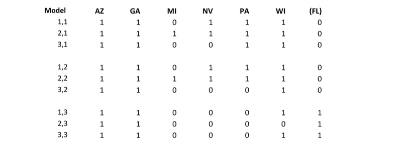
Weighting by total population without logarithm changes the results moderately. This weighting predicts flips in AZ, GA, WI _and FL_ (from Trump to Biden) for the simple formula and the (wwc+wpc+b+h)^2+avg formula; and in AZ, GA and FL only for the (wwc+wpc+b+h+avg)^2 formula. This is consistent with asking the regression to place the heaviest weight on explaining the outcomes in the largest urban counties. It is noticeable (and surprising to the authors) that even in the most extreme weighting of the data towards Biden’s urban strongholds, Wisconsin usually and AZ/GA always emerge as suspicious.
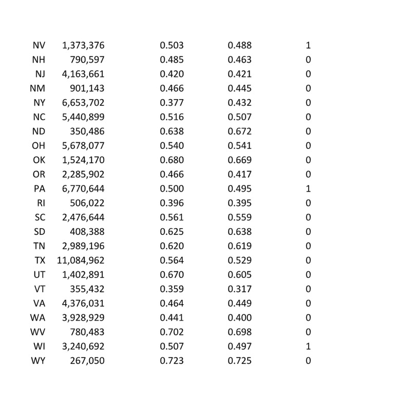
For reference the results of the nine combined model specifications (numbered as: model, weighting) are summarized in the following table, where “1” indicates that a model predicts a different result than observed.
6. The model places the burden of proof on fraud skeptics to explain why nearly all the states where fraud has been alleged, and only those states, have results inconsistent with statistical trends in the rest of the country.
If these allegations were simply sour grapes, we would expect to see more or less random errors in these states. No statistical model of the 2020 election would predict flips in 5 of 6 and near-flips in 6 of 6 randomly selected states unless it predicted flips for almost every state, or at least every close state.
Even if (in fact, particularly if) the fraud skeptic accepts the validity of the simple linear model of the election but still questions whether fraud is the most probable explanation for the gap between the model’s predictions for these states and the reported results, he must confront the burden of constructing five or six accounts of idiosyncratic voter behavior in particular states, and then explaining how it happens to be that these idiosyncrasies are synchronized. It is plausible to attribute one anomalous prediction to random error, and a second anomalous prediction to unique and irreproducible local events, but any rationalization that intends to introduce six coincidentally-aligned irreproducible local flukes should begin by apologizing for straining the credulity of its audience.
And in particular:
7. Our model highlights the importance of a systematic comparison of all counties in the US when trying to understand whether the contested states are actually unusual. Simply picking isolated comparison cities, or one-off comparisons to past elections, is a very inferior way of doing the comparison. This model takes this base intuition (which is actually good), but greatly improves it by making the comparison systematic. The fact that the contested states are mostly predicted to have been won by Trump using simple but powerful demographic models further adds weight to the existing evidence that these outcomes may have been altered by fraud.
One of the key advantages of this model is that it provides a systematic comparison of whether the contested states look unusual. This is far preferable to the general way commentary has proceeded, which has been generally to cherry pick individual cities or counties, assert that they are comparable control cases, and then do one-off comparisons with other years or locations. In some sense, this intuition is good, but the methodology is extremely poor – the chosen places may or may not be comparable in terms of demographics, and the choice to pick them may ignore other comparable controls. The regression setting avoids both problems — we consider all possible counties for comparison, and systematically examine the importance of the kinds of variables that people mostly think about in an ad hoc way.
Ross Douthat, for example, has opined on Twitter and in his New York Times column that two forms of direct evidence of fraud in Montgomery County, PA (both first published in Revolver) are irrelevant because Biden performed well in the Connecticut suburbs as well. But while Fairfax County, CT may be notable as a site to skinny-dip off Bill Buckley’s yacht — the event which marked Douthat’s initiation into the world of “insider intellectuals” — in the 2020 elections, events in the Connecticut suburbs were less memorable. Our model predicts a Trump two-party vote share of 39.865%, against reported 39.828% — not quite enough to flip the Nutmeg State. Our simple model finds Biden outperforming past Democratic performances with the college-educated white professional class not just in Connecticut or Pennsylvania but everywhere, and in all but five states the model is able to use those results to predict the winner. Douthat is free to reject any direct evidence of fraud in MontCo or elsewhere on its own merits, but the implicit argument that fraud is unlikely to have occurred in suburban PA (or AZ, GA, NV, or WI) because the results in these counties are similar to comparable counties elsewhere cannot be sustained, because the premise is false. These five states are not similar, they are idiosyncratic in some respect, and if Mr. Douthat wishes to remain a NY Times columnist in 2021 I suggest he get to work finding an innocent explanation for Biden’s statistically inexplicable strength in these five states.
The independent journalist Michael Tracey (and in Tracey’s defense it should be noted he has made heroic attempts to respond to a variety of theories about the 2020 election, some from quite obscure sources) has repeatedly made similar arguments against claims of fraud in metro Detroit, Milwaukee, and Philadelphia, on the grounds that Trump’s 2020 performance in these cities (like Trump’s urban performance elsewhere, notably in NYC) was actually an improvement on his 2016 results. Tracey takes for granted key aspects of our analysis here (that 2020 results should be consistent with other changes from past results in comparable counties in other states), but he has no numerical measure of “consistency” beyond pairwise comparisons of the cities in question: and when that measure is supplied, it becomes clear that while nationwide cities are predictably similar to other cities, suburbs predictably similar to other suburbs, in certain states the model’s predictions deviate from the reported outcome considerably: in these states Tracey is not free to argue that fraud is impossible because the county results are consistent with national patterns — in fact they are not consistent.
In aggregate, at the state level, anomalies larger than Biden’s margin of victory occurred somewhere in each of these five states: Douthat and Tracey are free to argue about what the nature of those anomalies was, in which counties they are most likely to have occurred, whether the best explanation is innocent or not, but they are not free to claim the anomalies occurred in every state, or that they are consistent with any general demographic pattern in changes in voter behavior in the 2020 election. By definition, they are not.
We do not mention Tracey and Douthat here to pick on them. Rather, they present in clear and intellectually honest form (honest, because it lays out its implicit empirical assumptions fairly unambiguously) a line of thinking that can be detected in nearly all skeptical responses to evidence of fraud.
CONCLUSIONS
This analysis has made formal an intuition that many people have had on an informal basis — namely, the contested states where Biden narrowly won showed strange voting patterns relative to what one might generally expect for those states, and relative to what one might expect on the basis of the final results in other key swing states (or plausibly even a sufficiently large number of “swing counties”). Our results show that this intuition can be made concrete — in the contested states of PA, WI, GA, AZ, and NV Biden’s vote share is implausible relative to both historical voting patterns in counties in those states, and with demographic trends in the 2020 election.
When a few simple rules suffice to explain almost all of the behavior of large numbers of people over enormous areas, when exceptions to the rules are too infrequent and small to leave any doubt about their operation, and various tweaks or additions to the rules don’t do much to improve, or even fundamentally change, the explanation (in other words: when a model is parsimonious, powerful, general, significant, and robust), then you can be confident in your results. The evidence presented here is very strong; not (by itself) overwhelming, but strong enough that with further corroboration of the statistical claims by evidence about particular counties and states, it must become overwhelming. Either the inhabitants of Arizona, Georgia, Pennsylvania, and (to a lesser extent) the three other contested swing states are totally unlike other Americans, and exempt from the statistical regularities that bind them, or rogue elements in the Democratic party have committed fraud on a scale that will permanently destroy America’s faith in elections unless their crime is quickly reversed and the guilty parties punished.
Read more at: Revolver.news and Trump.news.
by: News Editors
